Create EM Jobs via EMCLI

Found this saved but unpublished. Only 3 yrs late. 🙂

Basic flow:

Option 1: new job

1. list job types
2. describe job type and export to file
3. edit the exported file
4. create new job

Option 2: from existing job or from library job

1. list job type
2. describe job or describe job from library and export to file
3. edit the exported file
4. create new job

Other job related actions supported from EMCLI:

• Track progress
• create library jobs
• controlling job state – suspend, resume, stop, etc
• import/export

Refer to latest EMCLI documentation for more details.

Create Database using EMCLI Verbs

Tags

Automation, create database, deployment procedures, em12c, emcli, oracle enterprise manager, provisioning

Found this blog saved but unpublished. Posting it only 4 yrs late.

Quick note on running deployment procedures (DPs) using EMCLI verbs. Here we use the example of creating databases.

1. Run the DP once from the UI

2. Capture the data from this instance run

emcli get_instances -type=DBPROV

-> copy execution guid from your instance run

emcli get_instance_data -exec=<exec_guid> > instanceData.properties

3. Now modify the values in the properties file

4. submit the procedure with the modified properties file

emcli submit_procedure -input_file=data:modified-instanceData.properties -procedure=<procedure guid> -instance_name=emcli_test1

This will spit out output like:

Schedule not specified, defaults to immediate.

04CE42977F071862E0535C56F20A6A8F

Deployment procedure submitted successfully

5. Check status of DP using the instance ID printed below.

emcli get_instance_status -instance=04CE42977F071862E0535C56F20A6A8F

Here are the documentation links:

Provisioning Using EM CLI

https://docs.oracle.com/cd/E24628_01/em.121/e27046/emcli.htm#EMLCM12428

Example: Provisioning Oracle Database Software

https://docs.oracle.com/cd/E24628_01/em.121/e27046/emcli.htm#EMLCM11997

Understanding Docker Images and Layers

Tags

cloud, Docker, Docker, oracle, stateful, weblogic

Not so long ago, I presented a couple of sessions at the IOUG Collaborate 17 conference. During my session ‘Docker 101 for Oracle DBAs’ there were a bunch of questions regarding Docker images and the concept of layers and their benefits. So this blog basically summarizes the discussion I had with the audience during my session.

What are Docker Images and how do they compare to VM Images?

For anyone who has used VMs, the concept of a VM image is not new. A Docker image is very similar and serves the same purpose, that is, they are used to create containers, but that is where the similarity ends. While VM image is a single large file, a Docker image references a list of read-only layers that represent differences in the filesystem. These layers are stacked one over the other, as shown in the image below, and form the basis of the container root filesystem. The Docker storage driver stacks and maintains the different layers. The storage driver also manages sharing of layers across images. This makes building, pulling, pushing, and copying of images fast and saves on storage.

How are Images used to create Containers?

When you spawn a container (docker run <image-name>), each gets its own thin writable container layer, and all changes are stored in this container layer, this means that multiple containers can share access to the same underlying image and yet have their own data state.

When a container is deleted, all data stored is lost. For databases and data-centric apps, which require persistent storage, Docker allows mounting host’s filesystem directly into the container. This ensures that the data is persisted even after the container is deleted, and the data can be shared across multiple containers. Docker also allows mounting data volumes from external storage arrays and storage services like AWS EBS via its Docker Volume Plug-ins.

How do I find the layers of an Image?

The older versions of Docker provided `docker images –tree` which would show the tree view of all images and layers, unfortunately in the absence of that we have to look for other options.

For illustration, I am going to use an Oracle WebLogic server image I built. This image was built using multiple other images, each with their own set of layers.

You can see the total size of the image, currently 1.62GB, and the image ID.

Next, we will use the `docker history <image>` command to see the layers of this image. This output below shows all the layers that make up the weblogic image, but what are all these commands in the 2nd last column? For this, we have to refer to the dockerfile. Every instruction in the dockerfile creates a new layer, and since we used multiple dockerfiles to create the different images, this view shows the aggregate of all instructions run to build the final image we are using. Here is a good reference on how to write good dockerfiles.

While this information is good, it still doesn’t give us the hierarchical or tree view of images and layers. For this, we will use a hack. Run the following command to download an image from DockerHub, that will print out the tree view we want.

>> docker run –rm -v /var/run/docker.sock:/var/run/docker.sock nate/dockviz images -t

This view shows the same set of layers as the history command, but it also shows the lineage. If I focus on just the hierarchy of images & layers used to build by Oracle Weblogic image, I see that I used 4 different dockerfiles to build 4 different images. In fact, the last two images were derived from the same set of shared layers up till layer ‘bd54831efb16 Virtual Size: 1.2 GB’, after which the tree splits. Below is the hierarchy of images I built and used.

Now that I know the hierarchy of images being used, I can run ‘docker history’ command for each image and see its individual layers and the dockerfile instructions used to create them.

Once I completed mapping all layers to their respective images, I end up with a breakdown as follows.

Success!!

If you want to learn more about Docker and other container formats, take a look at my blog – Containers Deep Dive – LXC vs Docker

---

Shameless Plug: 

I currently work for Robin Systems and we provide an excellent container-based platform for both stateless and persistent stateful applications, especially for Big data applications and relational and no-SQL databases. This platform includes the 4 key components required to run stateful applications – containers (Docker and LXC), a scale-out block storage, virtual networking, and orchestration, and the platform can be deployed both on-premises on commodity hardware, or on public clouds like AWS.

Try our free community edition!

 

Linux: Analyze disk space full issues

Quick note to self.

The root partition on our servers at Robin Systems is restricted to 50G or 100G, mostly to ensure that we do not abuse it for caching or for storage of product artifacts. This also becomes a forcing function for me to keep my root partition clean and remove any redundant files. Whenever i get the ‘no space on device’ error, the first thing i want to do is to figure out the culprits. This is fairly easy to do:

du -h | sort -hr | head

This will spit out a reverse, sorted list of largest files in a given directory. I have also tried ncdu and i like it, but the above command saves me the trouble of installing new packages.

 

Can Containers Ease Cassandra Management Challenges?

Tags

cassandra, Docker, Docker, nosql database

This is a repost of my original blog on robin systems website.

Container-based virtualization and microservice architecture have taken the world by storm. Applications with a microservice architecture consist of a set of narrowly focused, independently deployable services, which are expected to fail. The advantage – increased agility and resilience. Agility since individual services can be updated and redeployed in isolation. While given the distributed nature of microservices, they can be deployed across different platforms and infrastructures, and the developers are forced to think about resilience from the ground up instead of as an afterthought. These are the defining principles for large web-scale and distributed applications, and web companies like Netflix, Twitter, Amazon, Google, etc have benefitted significantly with this paradigm.

Add containers to the mix. Containers are fast to deploy, allow bundling of all dependencies required for the application (break out of dependency hell), and are portable, which means you can truly write your application once and deploy it anywhere. Microservice architecture and containers, together, make applications that are faster to build and easier to maintain while having overall higher quality.

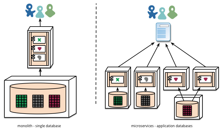
Image borrowed from Martin Fowler’s excellent blog:  http://martinfowler.com/articles/microservices.html

A major change forced by microservice architecture is decentralization of data. This means, unlike monolithic applications which prefer a single logical database for persistent data, microservices prefer letting each service manage its own database, either different instances of the same database technology, or entirely different database systems.

Unfortunately, databases are complex beasts, have strong dependence on storage, have customized solutions for HA, DR, and scaling, and if not tuned correctly will directly impact application performance. Consequently, the container ecosystem has largely ignored the heart of most applications: storage, and thus limit the benefits of container-based microservices due to the inability to containerize stateful & data heavy services like databases.

Majority of the container ecosystem vendors have mostly focussed on stateless applications. Why? Stateless applications are easy to deploy and manage. For example, its ability to respond to events by adding or removing instances of a service without needing to significantly change or reconfigure the application. For stateful applications, most container ecosystem vendors have focussed on orchestration, which only solves the problem of deployment and scale, or existing storage vendors have tried to retrofit their current solutions for containers via volume plug-ins to orchestration solutions. Unfortunately this is not sufficient.

To dive deeper into this, let’s take the example of Cassandra, a modern NoSQL database, and look at the scope of management challenges that need to be addressed.

Cassandra Management Challenges

While poor schema design and query performance remains as the most prevalent problem, it is rather application and use case specific, and requires an experienced database administrator to resolve. In fact, i would say most Cassandra admins, or any DBA for the matter, enjoy this task and pride themselves at being good at it.

The management tasks which Database admins would rather avoid and have automated are:

1. Low utilization and lack of consolidation
2. Complex cluster lifecycle management
3. Manual & cumbersome data management
4. Costly scaling

 

Let’s look at these one by one.

1. Low utilization and lack of consolidation

Cassandra clusters are, typically, created per use-case or SLA (read intensive, write intensive). In fact, the common practice is to give each team its own cluster. This would be an acceptable practise if clusters weren’t deployed on dedicated physical servers. In order to avoid performance and noisy neighbor issues, most enterprises stay away from virtual machines. This unfortunately means that underlying hardware has to be sized for peak workloads, leaving large amounts of spare capacity and idle hardware due to varying load profiles.

All this leads to poor utilization of infrastructure and very low consolidation ratios. This is a big issue for enterprises on both – on-premise and in the cloud.

Underutilized servers == Wasted money.

2. Complex Cluster Lifecycle Management

Given the need for physical infrastructure (compute, network, and storage), provisioning Cassandra clusters on premise can be time consuming and tedious. The hardest thing about this activity is estimating the read and write performance that will be delivered by the designed configuration, and hence often involves extensive schema design and performance testing on individual nodes.

Besides initial deployment, enterprises also have to cater to node failures. Failures are the norm, and have to be planned for from the get go. Node failures can be temporary or permanent and can be caused due to various reasons – hardware faults, power failure, natural disaster, operator errors, etc. While Cassandra is designed to withstand node failures, it still has to be resolved by adding replacement nodes, and it poses additional load on the remaining nodes for data rebalance – post failure and again post addition of new nodes.

1. Node A fails

2. Other nodes take on the load of node A

3. Node A is replaced with A1

4. Other nodes are loaded again as they stream data to node A1

 

3. Manual Data Management

Unlike traditional databases like Oracle, Cassandra does not come with utilities that automatically backup the database. Cassandra offers backup in terms of snapshots and incremental copies, but they are quite limited in features. Most notable limitations of snapshots are:

• Use hard-links to store point-in-time-copies
• Use the same disk as data files (compaction makes this worse)
• Are per node
• Do not include Schema backup
• No support for off-site relocation
• Have to be removed manually

Similarly, data recovery is fairly involved. Data recovery can be performed for two reasons:

1. to recover database from failures. For example, in case of data corruption, loss of data due to an incorrect `truncate table`, etc
2. to create a copy of it for other uses. For example, to create a clone for dev/test environments, to test schema changes, etc.

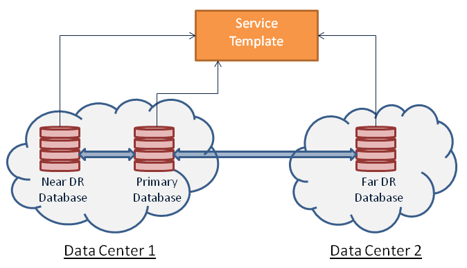
Typical steps to recover a node from data failures

In order to optimize for space used for backups, most enterprises will retain last 2 or 3 backups on the server but will move the rest to a remote location. This means based on the data sample needed, you maybe be able to restore locally on the server server or have to move files around from a remote source.

While Datastax Enterprise edition does provide notion of scheduled backups via OpsCenter, it still involves careful planning and execution.

4. Costly Scaling

With Cassandra’s ability to scale linearly, most administrators are quite accustomed to adding nodes (or scale out) to expand the size of clusters. With each node you gain additional processing power and data capacity. But while node addition is required to cater to steady increase in database usage, how does one handle transient spikes?

Let’s look at a scenario. Typically, once a year, most retail enterprises will go through the planning frenzy for Thanksgiving. Unfortunately, post that event, majority of the infrastructure would be idle or requires administrators to break the cluster and repurpose it for other uses. Wouldn’t it be interesting if there was a way to simply add/remove resources dynamically and scale the cluster up/down based on transient load demands?

Summary

Many enterprises have experimented with docker containers and open source orchestrators like mesos and kubernetes, but they soon discover that these tools along with their basic storage support in volume plugins only solve the problem of deployment and scale, but are unable to address challenges with container failover, data and performance management, and the ability to take care of transient workloads. In comes Robin Systems.

Robin is a container-based, application-centric, server and storage virtualization platform software which turns commodity hardware into a high-performance , elastic, and agile application/database consolidation platform. In particular, Robin is ideally suited for data-applications such as databases and Big data clusters as it provides most of the benefits of hypervisor-based virtualization but with bare-metal performance (up to 40% better than VMs) and application-level IO resource management capabilities such as minimum IOPS guarantee and max IOPS caps. Robin also dramatically simplifies data lifecycle management with features such as 1-click database snapshot, clones, and time-travel.

Join us for a webinar on Thursday, August 25 10am Pacific / 1pm Eastern to learn about how Robin’s converged, software-based infrastructure platform can make Cassandra management a breeze by addressing all aforementioned challenges.

 

Understanding Flash: Summary – NAND Flash Is A Royal Pain In The …

flashdba

So this is it – the last article in my mini-series on understanding flash. This is the bit where I draw it all together in a neat conclusion that makes you think, “Yes! That was worth reading”. No pressure eh?

So let me start with the conclusion first: as a storage medium, NAND flash is a royal pain in the ass.

Chaos

Why? Well, let’s look back at what we’ve learned in the previous 9 articles:

• Data stored in flash pages cannot be overwritten without an erase operation taking place first
• Erase operations affect entire blocks of flash pages instead of just the page you want to erase
• Erase operations are an order of magnitude slower than read and program (write) operations
• Flash media wears out and is limited by the number of program and erase operations (P/E Cycles) possible
• The performance of a flash package is unbalanced: for example,

View original post 953 more words

Oracle Private Database Cloud: Understanding the Resource Model

Tags

dbaas, em12c, emcli

In the public cloud parlance, consumers never provision to a specific server, instead they provision to a pool of infrastructure within a geographical region or data center. You would find this pattern in AWS, where you select Availability Zones or in Oracle Cloud, where you select the desired Data Center.

EM12c’s private database cloud follows a similar paradigm. It offers a two tier hierarchy in PaaS Infrastructure Zones, and Software Pools.

PaaS Infrastructure Zone (or Zone)

Zone is a logical grouping of cloud infrastructure resources (like servers, network, storage, etc) based on QOS, functional, departmental or geographic boundaries. For example, Finance Zone, East Coast Zone, etc. Cloud users or consumers provision into a Zone. A Zone is also used to enforce access control and chargeback/showback.

Database Software Pool (or Pool)

A  group of homogeneous clustered or non-clustered database resources exhibiting common characteristics. For example,
– Pool of 11.2 Database Oracle Homes (for dedicated databases)
– Pool of 12c Container Databases (for PDBs)

Okay now that we have covered some theory, lets take an example and walk through it. Our goal to offer a database service that is highly available and redundant across multiple data centers. This image below captures the situation well.

So lets get modeling.

A. Modeling Zones

1. We have two data centers – say one on the East Coast and the other on the West Coast. With this information, we could model two Zones based on the location dimension – East Coast Zone and West Coast Zone. As easy as this sounds, i don’t think putting all your hardware resources in a single grouping makes much sense.

2. Its likely that we have servers from different vendors, with different architectures, etc. Assume we own a few Exadata, some commodity servers, some SPARC servers, some VMs, etc. To accommodate this, we can update our model with the hardware dimension – East Coast-Exadata Zone, East Coast-Commodity Zone, East Coast-Sparc Zone, etc.

3. Now typically, hardware is rolled out to host applications, databases, etc. Applications have a lifecycle, they start in the development environment, then move to test, stage, performance, and finally production. Separate hardware is allocated for each of these environments, each with different characteristics – performance, cost, redundancy, etc Again, we can update our model with this new lifecycle dimension – East Coast-Exadata-Development Zone, East Coast-Exadata-Production Zone, etc

It is important to note, that all of the above dimensions are derived based on my experience with a bunch of customers. You are not required to use all of them, and it always helps to keep things simple. Lets look at pools next.

B. Modeling Pools

Pools are more software and platform centric and thus can be modeled based on various dimensions. Common dimensions are:

• Service Type: EM supports 3 service types – database, schema, and pluggable databases
• Version: This is the database software / Oracle home version
• Platform: This corresponds to operating systems like linux x86, solaris, hp-ux, etc
• High Availability: This represents if the infrastructure is RAC or SI (single instance)
• Disaster Recovery: Indicates if the pool will be used to host standby databases or just primary

So the naming format for Pools could be like this: 
<Service_Type>-<Version>-<Platform>-<HA>-<DR> 

Some examples: 
DB-11204-linux-RAC, DB-11204-linux-SI-STANDBY, PDB-12102-RAC, etc

Again, as i said before these are mere suggestions, and it is really up to you to decide which works best for you.

Lets come back to our example from above. If i try to implement the resource model so as to deploy a highly available and redundant database service, it would look something like this:

The zone name should indicate its composition. In the pool name, i skip the platform part since i am using Exadata and hence i assume Linux automatically. If you are using VMs or commodity hardware you may want to specify the platform as well. So my pools are composed of GI clusters deployed on Exadata compute nodes and the DB Oracle home pre-provisioned. Note a pool can contain multiple clusters. At the time of provisioning, the placement algorithm ensures that the requested database is created on a cluster with least utilized nodes. This is the power of automation provided by EM 12c.

In summary, with the EM12c resource model, cloud providers have the ability to organize and manage their infrastructure the way they would like, while keeping the consumer experience simple and intuitive.

References:

Screenwatch: Build Service Catalogs with EM12c DBaaS

Oracle Private Database Cloud: Defining Database Sizes in the Service Catalog

Tags

database as a service, em12c, emcli, private cloud

Latest release of cloud plug-in (part of EM12c R4 Plug-in Update 1) brings the ability to define sizes for database cloud services (Schema and PDB services already support definition of size). Prior to this ability, customers were required to define a new template for each size – small, medium, large, etc. This will help in significantly reducing the number of templates required.

So lets see how to use them.

1. The CRUD operations for database size are performed via emcli verbs. To create a new size, we run:

./emcli create_database_size -name=Tiny -description="tiny size" 
        -attributes="cpu:2;storage:20;memory:2"

The 4 attributes supported for size are – cpu, memory, processes, & storage. All attributes are optional, and minimum name and description need to be provided.

To list all sizes, we run:

./emcli list_database_sizes
 ____________________________________________
 Name:tiny
 Description:tiny size
 CPU(cores):2
 Memory(GB):2
 Processes(COUNT):Not Specified
 Storage(GB):20
 ____________________________________________

Had this size been assigned to any service templates, we could have provided the -details flag and gotten that list as well.

Editing this size is equally easy. We run:

./emcli update_database_size -name=tiny 
        -description="Tiny database size" 
        -attributes="storage:remove;processes:500"
 ____________________________________________
 Name:tiny
 Description:Tiny database size
 CPU(cores):2
 Memory(GB):2
 Processes(COUNT):500
 Storage(GB):Not Specified
 ____________________________________________

Few things to notice are:

• name is the only fixed identifier, both attributes and description can be changed
• to remove an attribute, set its value to remove
• to set new attribute values, or change existing one, simply specify the new values

Finally, to delete a size, we run:

./emcli delete_database_size -name=tiny
 Are you sure you want to to delete?(yes/no)
 yes
 Database size tiny has successfully been deleted

Since delete is a destructive operation operation, you get the “Are you sure?” prompt.

2. Once sizes are defined, we can see them while creating or editing service templates. Note that by default, no sizes are attached with the service template. The administrator needs to explicitly associate a size with the template, as shown in the screenshot below.

3. Once the association is complete, and the template is saved. Any cloud consumer accessing the template via the cloud portal will see size as an additional input.

If you are using REST APIs, then database size will have to be provided as an additional input to the POST request.

A commonly asked question is that how are these values enforced? The answer depends on the the type of attribute:

• cpu – this translates to cpu_count and is set as the DB init parameter
• memory – this translates to memory_target and set as DB init parameter (This is a good time to mention that the memory attribute is only supported for DB version 11g and above. Other attributes work for 10g and above.)
• storage – this is used only for monitoring purposes, and not enforced. So at the time of provisioning we ensure that the storage requirements for the service are within the quota limits of the consumer, but these limits are not set on the database.
• processes – this is set as DB init parameter

In summary, the ability to define size as an external entity will help drastically reduce the number of templates required to be defined by the cloud administrators.

Additional Resources:

EMCLI Documentation

Discover and Promote Oracle Homes as EM Targets

Tags

add target, em12c, emcli, job system, oracle home

Typically, Oracle Homes are discovered and promoted as targets automatically along with guided flows for addition of primary targets like databases, weblogic domains, etc, but there might be instances (not very often) where you need to discover the Homes standalone.

There are two ways to do this – from the GUI and using EMCLI verbs

A. From GUI

The steps are as follows:

1. Goto Enterprise->Job->Activity menu item
2. Here select the job type ‘Discover Promote Oracle Home Target’ and click Go
3. Provide the obvious inputs like name, list of hosts, etc, but the most important tab is that of ‘Parameters’. Here you are required to provide 3 inputs:
   1. Path to Oracle Home/Inventory/Composite Home/Middleware Home you want to manage
   2. The type of entity you want to manage. Your options are – Oracle Home, Inventory, Composite Home, or Middleware Home
   3. The action – discover and promote, or just discover [I almost always select the former]

That’s it. All remaining tabs are optional. Once the job is submitted, it usually takes a few seconds to complete. The output of the job clearly lists all the Oracle Homes discovered and the target names created for these Homes in EM.

B. Using EMCLI

1. First we describe the job type to get the list of required inputs

./emcli describe_job_type 
        -job_type=discoverPromoteOHTargets  > inputs.prop

If the explanation of the required fields is not sufficient, you can additionally pass the -verbose flag to get more details.

Now update the inputs.prop file with the relevant values. My file looks like this (changed values in red):

# Description: (Optional) The user specified name of the job
name=promote_OH

# Description: (Optional) The job type for this job
type=discoverPromoteOHTargets

# Description: (Optional) The user specified description of the job
description=

# Description: The job owner. The job owner is the user who creates the job.
# Default: the logged in user
# The job owner information displayed here is for documentation only 
# and user is not expected to change it.
owner=

# Description: (Optional) The kind of job
# Legal Values: active, library
kind=active


# Fill in the target list before submitting.
# For Example:
#     target_list=MyTarget:cluster
target_list=abc.example.com:host

# Description: The type of targets to use for this job
targetType=host

# Description: (Required) Enter the action you want to perform.
# To run only discovery on the target, use : disc.To run discovery 
# and promotion on target to managed status, use : promote
variable.loc_action=promote

# Description: (Required) Enter the type of search to be performed. 
# All the homes in the Inventory/Middleware Home will be managed.
# For discovering Oracle Home, use : oh.For discovering Oracle Home's
# in inventory , use : inv.For discovering Oracle Home's in 
# middleware home, use : mwh
variable.loc_type=inv

# Description: (Optional) Enter Path to Oracle Home/Inventory/
# Composite Home/Middleware Home you want to manage.
variable.location=/u01/foo/oraInventory

# Description: (Optional) Notify the job owner when a selected state occurs
# Allowed Values:  SCHEDULED, RUNNING, ACTION_REQUIRED, SUSPENDED, SUCCEEDED, PROBLEMS
notification=

Note, i submit my job against a single host target, but you can provide a long comma separated list of <target_name>:<target_type>. Now we submit the job by passing the above inputs.prop file as input.

emcli create_job -input_file=property_file:inputs.prop
Creation of job "PROMOTE_OH" was successful.

Since the EM12c job system is asynchronous, the emcli verb will submit the job and return control almost instantly. We need to run different set of emcli verbs to get job progress.

emcli get_jobs -name=PROMOTE_OH
Name        Type                      Job ID                            Execution ID
      Scheduled            Completed            TZ Offset  Status     Status ID  Owner   Target Type
  Target Name
PROMOTE_OH  discoverPromoteOHTargets  10FBD71FF8C70205E050F00A07B46726  10FBD71FF8C90205E050F00A07B46726  
2015-03-10 22:34:33  2015-03-10 22:34:37  GMT-07:00  Succeeded  5          SYSMAN  host
  abc.example.com

The output is ill formatted, but the only 2 fields we care about are – Execution ID and the Status. Since this is a fairly quick job, the status is shown as Succeeded. If i wanted to view the output, i would run another emcli command, and for this we need the execution ID.

emcli get_job_execution_detail 
      -execution=10FBD71FF8C90205E050F00A07B46726 -xml -showOutput
<?xml version = '1.0' encoding = 'UTF-8'?>
<jobExecution jobOwner="SYSMAN" status="5" startTime="2015-03-11 05:34:34.0" id="10FBD71FF8C90205E05
0F00A07B46726" jobName="PROMOTE_OH" statusBucket="-5">
   <TargetList>
      <target name="abc.example.com" type="host" hostName="abc.example.com"/>
   </TargetList>
   <steps>
      <step command="DiscoverAndPromoteOH" status="5" name="RunCustomDiscovery" startTime="2015.03.1
0 22:34:34" endTime="2015.03.10 22:34:37" timezoneRegion="-07:00" stepId="825682" stepType="1" jobTy
pe="discoverPromoteOHTargets" stepNlsId="discoverPromoteOHTargets_RunCustomDiscovery" stepDefaultNam
e="RunCustomDiscovery" target="">
         <stepOutput>
            <output>Discovered Oracle Home Target 'OraDB12Home1_11_abc.example.com' with home
 location - /u01/db12/product/12.1.0/dbhome_1 in Inventory /u01/foo/oraInventory.
Successfully created 1 new Oracle Home Targets.
Succesfully added discovered homes matching given criteria.</output>
         </stepOutput>
      </step>
   </steps>
</jobExecution>

The output clearly states the outcome of the job, and if i check my all targets page, i will find the new Oracle Home target.

In summary, while there may not be many reasons to just discover and promote standalone Oracle Homes, if you ever need to do it, this blog tells you how to do it both via the GUI and EMCLI.

Understanding Agent Resynchronization

Tags

agent, em12c, resynchronization

Agent Resynchronization (resync) is an important topic but often misunderstood or misused. In this Q&A styled blog, I discuss how and when it is appropriate to use agent resynchronization.

What is Agent Resynchronization?

Management Agent can be reconfigured using target information present in the Management Repository. Resynchronization pushes all targets and related information from the Management Repository to the Management Agent and then unblocks the Agent.

 Why do agents need to be re-synchronized?

There are two primary reasons why you may need to use agent resynchronization:

1. Agent is blocked

An agent is blocked whenever it is out-of-sync with the repository. This, typically, can happen due to a corrupt targets.xml, missing files and directories, and bugs in the code (they are rare but few do exist 🙂 ) that can leave the plug-in inventories in a strange state. In this condition, the OMS rejects all heartbeat or upload requests from the blocked agent. This means, the blocked agent will not be able to upload any alerts or metric data to the OMS, but it does continue to collect monitoring data. This is useful as once the agent is resynchronized, no monitoring data is lost.

2. Agent is lost and has to be reinstalled

This could be considered to be a special case of agent blocked condition, but it is worth discussing separately. If an agent host or file system is ever lost, the recommended way to reinstall it is by cloning from a reference install. This not only recovers the agent, but avoids having to track and reapply customizations and patches.

Note: It is important to retain the same port when reinstalling the agent.

Agent resync when run on a reinstalled agent, reconfigures it using target information present in the repository. The OMS detects that the agent has been re-installed and blocks it temporarily to prevent the auto-discovered targets in the re-installed agent from overwriting previous customizations.

Note: NEVER, NEVER, combine agent recovery with upgrade! If you lose your agent, recover it first using the original version, and then upgrade it to the new release.

Which interfaces are available for this operation?

There are two interfaces that will allow you to perform agent resync.

1. The Enterprise Manager Console

a. Navigate to Setup->Manage Cloud Control->Agents to view list of all agents

b. Select the desired agent and visit its home page

c. Finally, select the ‘Resynchronization…’ option from the agent menu

2. EMCLI

The agent can also be resynchronized via EMCLI. The command is as follows:

>> emcli resyncAgent -agent="Agent Host:Port"

How long does it take to resynchronize an agent?

This is a popular question, but unfortunately there is no straight answer for it. The time for resynchronization depends on the amount of data stored in the repository about the agent. When this action is invoked, the OMS does not consult the agent – it just asks agent to delete everything first, and then pushes the known state to it. Majority of the time is spent in pushing the plug-in content. So the more plug-ins deployed to the agent, the longer it takes. Metric Extensions and Configuration Extensions deployed to the agent would also contribute to the time.

Additional  Resources:

Upgrading  Oracle Management Agents

Back Up and Recover Enterprise Manager